Model Course

Task:  Try to understand the model in general and the provided implementation.

The following picture gives you an overview of the supply chain and the decisions that have to be taken. Note that demand and available resources are dependent on the scenarios.

The following graphic informally illustrates the structure of our supply chain.

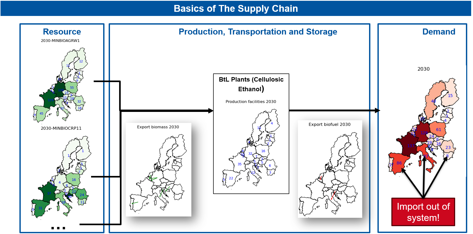
The supply chain is composed of the following five steps:

1. Calculate the availability of different types of biomass.
2. Export and transport them to production plants in various countries.
3. Convert the biomass into biofuels at these production plants.
4. Export the biofuels to demand points.
5. If the produced biofuel is insufficient, imports from outside the system can meet the remaining demand. These imports are modelled as being highly expensive, as the case study aims to assess whether the EU can operate self-sufficiently.

To integrate this supply chain into our Python model, we begin by modelling it using the following graph structure:

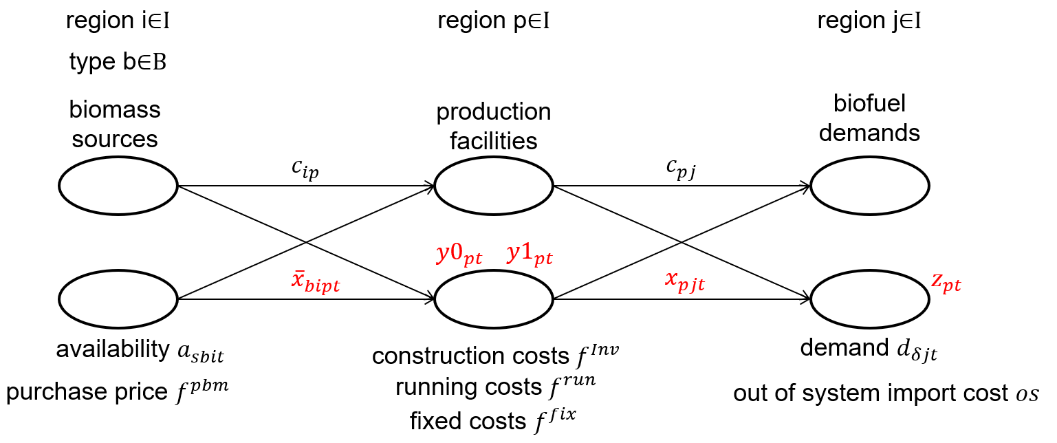
Using this graph as a foundation, we develop an MIP model to simulate the supply chain under a fixed scenario, meaning it does not account for uncertainty for now. Below, we first outline the Indices, Parameters, and Decision Variables, followed by a detailed presentation of the MIP formulation.

Indices:

\( b \in B \) set of biomass types

\( s \in S \) set of biomass scenarios

\( \delta \in D \) set of demand scenarios

\( t \in T \) set of time periods  (Time period 1 model's 2030 and the last 2050)

\( i,j,p \in I \) set of regions, we use \(i\) to model regions with biomass, \(p\) for regions we are building facilities and \(j\) for the demand

Decision Variables:

\( \overline{x}_{bipt}\) Transport quantity of biomass \( b \) from region \( i \) to facility \( p \) at time \( t \)
\(x_{pjt}\)  Transport quantity of biofuel from facility \( p \) to region \( j \) at time \( t \)
\(y_{p0}\)   number of open production facilitys \( p \) at time 2030
\(y_{p1}\)   number of open production facilitys \( p \) at time 2040
\(z_{pt}\)   imports from outside the system to region  \( j \) at time \( t \)

Scenario Parameters:

\( s\) selected biomass scenario
\( \delta\) selected demand scenario
\( r\) allow reinvestment \( r=1 \) , else \( r=0 \)

Parameters:

\( a_{sbit}\) maximum available amount of biomass \( b \) in region \( i \) at the time \( t \) in scenario \( s \)
\( f_{sbit}^{pbm}\) purchase price for biomass \( b \) in region \( i \) at the time \( t  \) in scenario \( s \) 
\( HV_{b}\)  heating value of biomass \( b \)
\( HV^{bf}\) heating value of biofuel
\( c_{ij}\) distance between region \( i \) and \( j \)
\( t^{bf}\) transport cost for biofuel
\( t^{bm}\) transport cost for biomass
\( Conv\)  conversion factor from units of biomass to units of biofuel
\( d_{\delta jt}\) demand in region \( j \) at the time \( t \) for demand scenario \( \delta \)
\( f^{fix}\) periodic fixed operating costs for a facility
\( f^{inv}\) construction costs for facility
\( f^{run}\) periodic variable operating costs for running a facility
\( s^{max}\) maximum capacity of a facility
\( UT\) uptime per period in which the facility is producing
\( LT\) lifetime of a facility
\( os\)  cost to import biofuel from outside the system

Target Function:

\( min \sum_{t \in T}  (BC_t + TC_t + PC_t + OC_t) \)

BC = Biomass acquisition cost. Individual prices for each biomass.

\( BC_t = \sum_{b \in B}\sum_{i \in I}\sum_{p \in I}f_{bit}^{pbm}{\overline{x}}_{bipt}  \)

TC = Transport cost. As prices are given in tonnes per km, individual heating values of each biomass or respective the fuel are needed. As the model, decision variables are in PJ.

\( TC_t = \sum_{b \in B}\sum_{i \in I}\sum_{p \in I} t^{bm} c_{ip}  \dfrac{{\overline{x}}_{bipt}}{HV_{b}} + \sum_{p \in I}\sum_{j \in I} t^{bf} c_{pj} \dfrac{x_{pjt}}{HV^{bf}} \)

PC = Production cost. Takes the individual production cost of biofuel as well as investment values. (Note: The function written here is actually not completely correct, as y0 and y1 have to be used depending on \(t\)!)

\( PC_t = \sum_{p \in I}\sum_{j \in I} f^{run} x_{pjt} +  \sum_{p \in I}^{}{(\frac{f^{Inv}}{LT}+f^{fix})y_{pt}} \)

OC = Out of system import cost.

\( OC_t = \sum_{j \in I} z_{jt}  os \) 

Constraints:

\( \sum_{p \in I}{\overline{x}}_{bipt} \leq a_{sbit}  \forall\ b \in B,\ i \in I,\ t \in T \)

(1) Compliance with the existing biomass volume limits  

\( \sum_{b \in B}\sum_{i \in I}{\overline{x}}_{bipt} - Conv \sum_{j \in I}x_{pjt} \geq 0\  \forall\ p \in I,\ t \in T \)

(2) Energy conservation in the production facilities

\( z_{jt} + \sum_{p \in I} x_{pjt} \geq d_{\delta jt}\ \forall\ j \in I,\ t \in T \)

(3) Meeting the demand of biofuels

\( s^{max} * UT * y0_{pt} \geq \sum_{j \in I} x_{pjt}\ \forall\ p \in I,\ t \in \{2030,..,2039\} \)
\( s^{max} * UT * y1_{pt} \geq \sum_{j \in I} x_{pjt}\ \forall\ p \in I,\ t \in t \in \{2040,..,2050\} \)

(4,5) Used capacity must be less than the available capacity

\( y1_{p} \geq y0_{p}\ \forall\ p \in I, \text{if } r=1 \)
\( y1_{p} = y0_{p}\ \forall\ p \in I, \text{if } r=0 \)

(6,7) Non-demolition constraint for all facilities, if no reinvestment is allowed. Also limiting reinvestment.

\( \overline{x}_{bipt} \geq 0\ \forall\ b \in B,\ i, p \in I,\ t \in T \)
\( x_{pjt} \geq 0\ \forall\ p, j \in I,\ t \in T \)

(8,9) Non negativity

\( y0_{p} \in \mathbb{N}_{0}\ \forall\ p \in I \)
\( y1_{p} \in \mathbb{N}_{0}\ \forall\ p \in I \)

(10,11) Production facilities are integers