Model Course

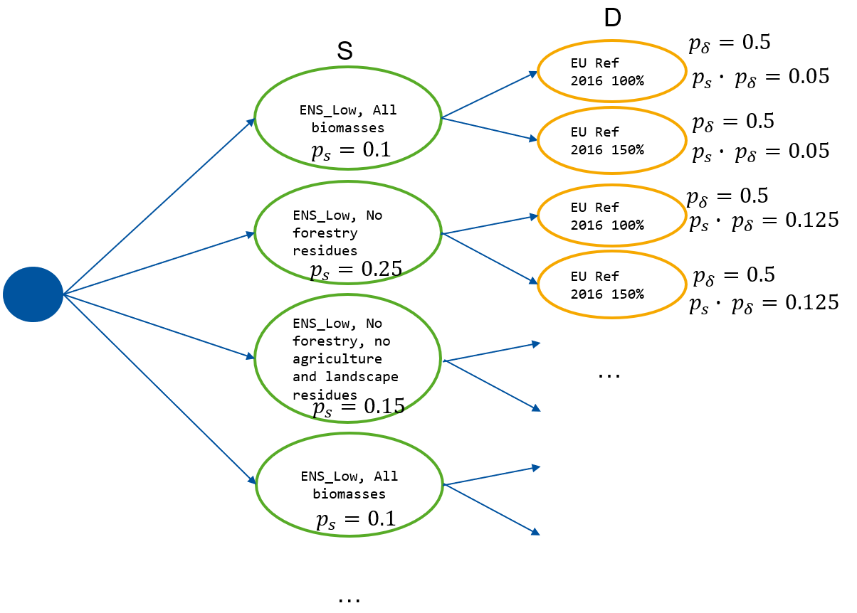
We can depict our scenarios in a scenarios tree. This can be read like this. For each biomass scenario, both demand scenarios can happen. Thus, with 6 biomass scenarios and 2 demand scenarios, we get a total of 12 scenarios. The probability of each scenario happening is the probability of the scenarios multiplied.

Scenario Tree:

To make a meaningful recourse model, we have to separate our decision in the model into here-and-now and wait-and-see decisions. In our case, just the initial investment \( y0 \) are to be taken now. All other decision are taken after the scenarios happen, thus are recourse decision.

To make our model, we need to extend all our recourse decision variables with a new index for the scenario. As we have two uncertainties, we can also introduce two new indices, and the combination of the describes one scenario.

E.g. we need to extend

 \( \overline{x}_{bipt} \) Transport quantity of biomass \( b \) from region \( i \) to facility \( p \) in period \( t \)

to

 \( \overline{x}_{s \delta bipt} \) Transport quantity in biomass scenario s and in demand scenario \( \delta \)  of biomass \( b \) from region \( i \) to facility \( p \) in period \( t \)

Apply this procedure to all relevant variables and adjust the constraints as necessary. If you are uncertain about how to proceed, refer to the stochastic model described in the lecture slides.

The target function should be then here-and-now part (100%) + the wait-and-see part of each scenario \(s \delta\) by its probability \(p_s \cdot p_{\delta} \).

Task: Implement the model in the given Jupyter notebook cell. It will probably help you to do the extension first on paper.