
Case Study

From 2030 onwards biofuels of the second generation could make a substantial contribution to satisfy the demand for climate-neutral mobility. You should create an example supply chain to satisfy the future demand for biofuels (2030 to 2050) and assess if this approach is feasible and how much it would cost. 
You should model the supply chain for a range of European countries and assume that you can access all available biomass. The focus should be that the fuel production does not compete with food production. This favours e.g. agricultural waste, miscanthus, switchgrass or sawdust.
 
For each region, you can assume that you have a demand for the years 2030 to 2050.  All demand has to be satisfied.  The demand for fuel as well as the availability of biofuel is given in the same unit (PJ). We assume that in the production, we have the same conversion factor for all biomasses.
 
You should calculate in which regions it is most advantageous to create the production facilities. Building a facility has a certain investment cost. The facility can run for a certain amount of time. Once a production facility is built, there are costs to run it each year. The costs to build and run the facilities are given for an example facility. Once it is created, it cannot be expanded. (Note: for simplicity reason, we will not discount investments, calculate net present values, etc. We also do not consider that in different countries building and running the plant would have different costs.)
 
The transportation between the location of the biomass and the facilities is done by truck. The same applies to the transport between the facility and the regions with the demand. You can assume linear costs for the transportation, relating to distance travelled and tonne transported. Each biomass, as well as the biofuel, has a heating value that gives a weight that is attributed to a PJ of that biomass/biofuel. Transporting fuel is more expensive than transporting biomass.
 
The following chapters will guide you through the implementation.
  1. Create a mixed-integer linear program (MILP) model that models this supply chain.
  2. In the following quiz, we will ask you what the equivalents between the standard 2-Stage Warehouse Location Problem (WLP) and the supply chain are. You could also use this quiz as a help if you do not know how to model the supply chain directly. (Note: You should still try before doing the quiz!)
  3. Read through the data chapter and understand which data is used and how you can read it into a Python program.
  4. Take the given implementation, run it and analyse the results.
  5. Implement a second target function and create the Pareto front.
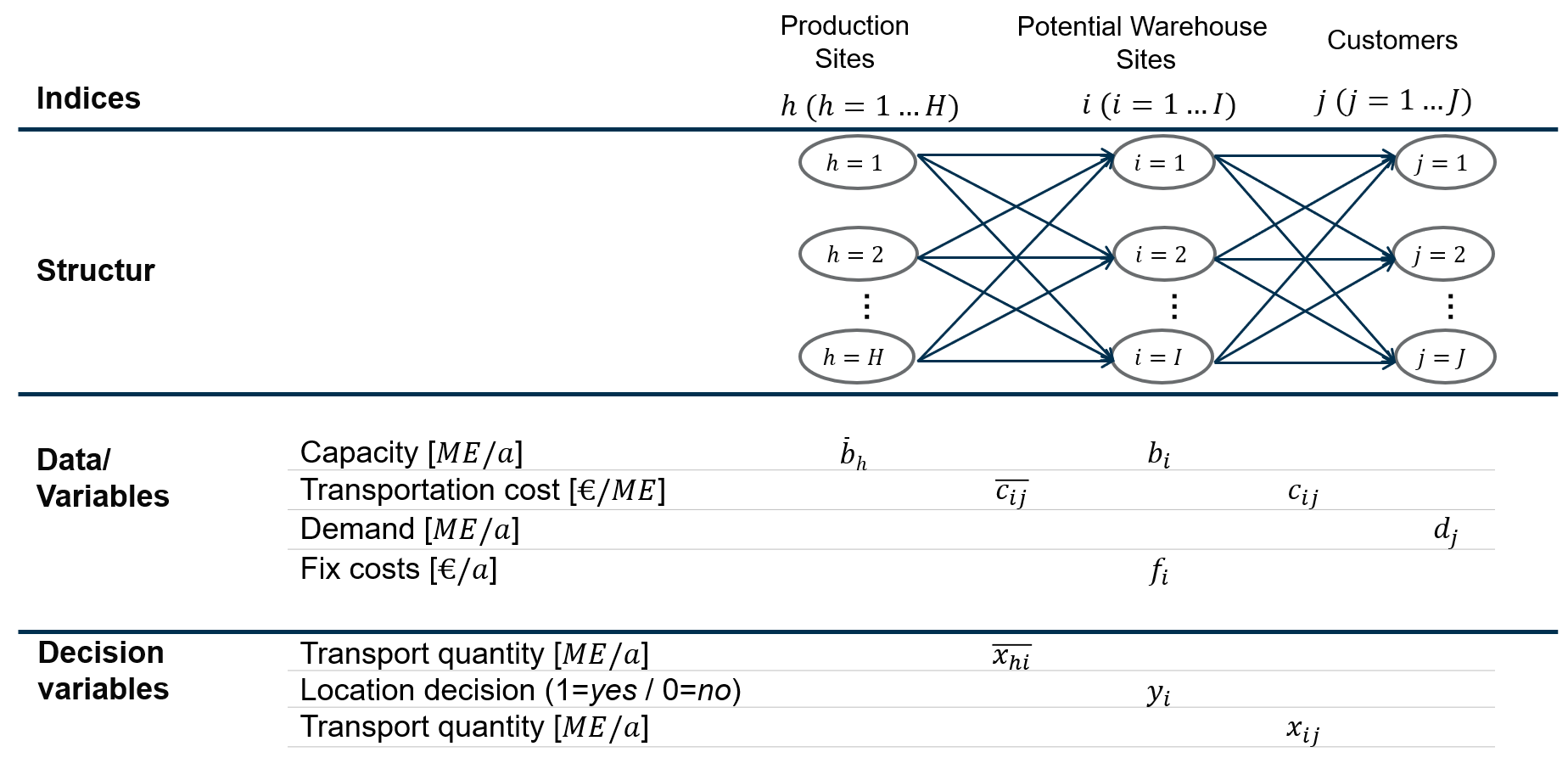
As a help, for the first step, we will now provide you the two-stage Warehouse Location Problem. It can be adapted with only a few steps to model the supply chain above.
 

Graphical representation of the 2-Stage WLP, with all variables and indices highlighted

Indices:

Set of production sites: \(h \in H\) 

Set of potential warehouse sites: \(i \in I\) 

Set of customers: \(j \in J\) 

Decision Variables:

\( \overline{x}_{hi} \) Transport quantity from production site \( h \) to facility \( i \)

\( x_{ij} \) Transport quantity from warehouse \( i \) to customer \( j \)

\( y_{p} \) Location decision for warehouse  \( i \)

Parameters:

\(  \overline{b}_{h} \)  Capacity of production site \( h \)

\(  b_{i} \)  Capacity of warehouse \( i \) 

\( \overline{c}_{hi} \) Transport cost from production site \( h \) to facility \( i \)

\( c_{ij} \) Transport cost from warehouse \( i \) to customer \( j \)

\(  \overline{d}_{j} \)  Demand of customer \( j \) 

\(  f_{i} \)  Fixed cost of warehouse \( i \) 

Target Function:

\( Min Z= \sum_{h,i} \overline{c}_{hi}  \overline{x}_{hi} + \sum_{i,j}  c_{ij} x_{ij} + \sum_{i} f_i y_i \)

Constraints:

No more can be supplied from a production site than capacity is available:

\( \sum_{i=1}^{I} \overline{x}_{hi} \leq \overline{b}_h,  \forall h \)

The outflow from the warehouses is equal to the inflow into the warehouse:

\( \sum_{h=1}^{H} \overline{x}_{hi}  - \sum_{j=1}^{J} x_{ij} = 0,  \forall i \)

Capacity limitation of the warehouses must be respected:

\( \sum_{j=1}^{J} x_{ij} \leq b_i y_i,  \forall i \)

Meeting demands for all customers:

\( \sum_{i=1}^{I} x_{ij} = d_j,  \forall j \)

Non-negativity condition:

\( \overline{x}_{hi} \geq 0,  \forall h,i \)

Non-negativity condition:

\( x_{ij} \geq 0,  \forall i,j \)

Binary condition:

\( y_i \in \{0,1\},  \forall i \)

Hai completato il 65% della lezione
65%