
Model Course
Multi Objective Extension
The model till now only looks at the economic impact. You are now tasked to also consider an environmental component.
Land-use and nitrogen data
In the paper, we find data to land use intensity and nitrogen intensity for energy crops. The authors came up with a weighting measurement. For agriculture and landscape residues, forestry and waste biomass, we assume that there is no land use or use of nitrogen. We provide this data in the form of an Excel sheet.
Fritsche, U. R., Berndes, G., Cowie, A. L., Dale,. V. H., Kline, K. L., Johnson,F. X., et al. (2017). Global Land Outlook: Energy and Land Use. International Renewable Energy Agency (IRENA)
Create a target function using land use as an optimization objective. Then read the explanations underneath and create a Pareto front.
The epsilon constraint method
This will give us a second target function \(f2\) next to the economic one \(f1\). You will now not find a solution that is optimal for \(f1\) as well as for \(f2\). The two target functions are conflicting. But what we can do is find Pareto optimal solutions. (Note: We suggest some extra self study here, if you are not aware what Pareto optimality/efficiency is.)
In short, we want to see all the solutions that are along the boarder between the solvable space (the blue line in the diagram underneath). There might be other solutions in the orange part. However, we could always improve the solution further for at least one of the target functions by moving to the blue line.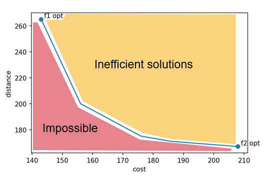
With the Epsilon constraint method, we can calculate a set of solutions that will resemble the Pareto front. This is an approximation and not a completely correct method, but it suffices in most cases. As it is straightforward and easy to implement, this is preferred over exact solutions.
- Calculate \(min f1\) and retrieve \(x_{opt1}\).
- Calculate \(min f2\) and retrieve \(x_{opt2}\).
- Take one of the two functions as your main function (e.g. \(f1\)).
- Select a value \(m \in N^+\) on how many parts you want to split your Pareto front in. The higher \( m \) is, the more accurate is your front.
- Calculate \( r = f_2(x_{opt1}) - f_2(x_{opt2}) \).
- Iteration over \( i \) with \( i \leq m, i \in N\):
- Calculate \(\epsilon_i = f_2(x_{opt2}) + \dfrac{r}{m} * i \).
- Introduce \(f2 \leq \epsilon_i \) as a new constraint and solve the new model.
- Save the optimal solution as one point.
- Use all the saved points from the iteration to create the Pareto front.
- Extend your model for a land-use target function
- Watch the video and look at the example code
- Calculate a Pareto front!
Implementation Hints:
- In the code the positions where you should do your implementation are marked with TODO, just in data_handler.py and model.py there are things to be done.
- If you plot your Pareto front, do not include the value of land-use optimal, as it is so far away from the other values that it makes the rest unreadable.
- Do not restrict your model to an epsilon that is exactly optimal to one of the two target functions. Gurobi is not 100% numerical stable and might declare the model unsolvable.
- 10 iterations of the Pareto front values (\(m\)) are enough, no need to go to the standard of 100.