4a. Tutorial - Optimal Unit Commitment
| Website: | RUB Moodle |
| Kurs: | Case Study "Novel flexibility options in the German electricity grid" |
| Buch: | 4a. Tutorial - Optimal Unit Commitment |
| Gedruckt von: | Gast |
| Datum: | Mittwoch, 18. März 2026, 06:36 |
Introduction
In this tutorial, you will learn how to use backbone for optimizing the unit commitment in an energy system. Information on the theoretical background of optimization and unit commitment you can find in the videos LINK.
Backbone is an open source energy system optimization model, developed by the VTT in Finnland (see https://gitlab.vtt.fi/backbone/backbone and [1]). Backbone is programmed in GAMS. You can build a model of your energy system and then use backbone to find the cost optimal solution of your system.
Note: The case study works best on Windows machines. However, it also can be completed on Mac or Linux machines. The only drawback here is, that the automated export of results to Excel does not work. To manually export data to Excel, you must use the export button in GAMS studio (more on that later on).
[1] Helistö, N.; Kiviluoma, J.; Ikäheimo, J.; Rasku, T.; Rinne, E.; O’Dwyer, C.; Li, R.; Flynn, D. Backbone—An Adaptable Energy Systems Modelling Framework. Energies 2019, 12, 3388. https://doi.org/10.3390/en12173388
System Overview
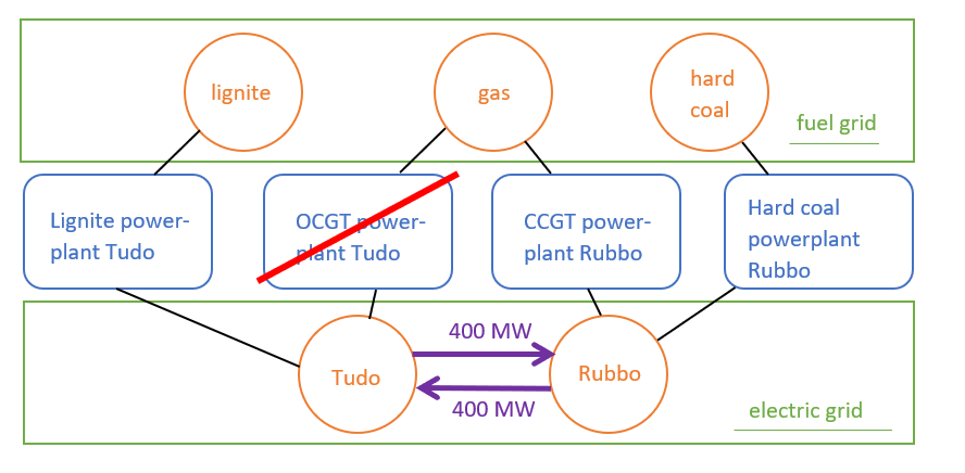
In this tutorial, we will continue to use the energy system of Tudo and Rubbo. Unfortunately, the OCGT plant is broken down and cannot be used anymore. To run an energy system optimization with backbone, we have to perform the following three steps:
- Fill in the backbone input file in excel.
- Run backbone.
- Display and interpret results.

Fill the backbone input excel
The
following tasks aim to help you with filling in this input data file. First, you should download the template file "Input data Tutorial unit commitment" from moodle and open it in Excel or LibreOffice. In this part of the tutorial, we will only fill in the blue sheets. Be careful to use the exact
names for girds, nodes and unit as they are defined in the yellow sheets.
p_gn
First, we will take a look at the table p_gn. Here, nodes are connected to the grids they belong to. Write all nodes in the column “node” and write the corresponding grids in the column “grid”. The parameter “nodeBalance” determines, whether input and output must always be equal for the node. For all nodes, where energy balance is required, write 1 in the column “nodeBalance”, for all other nodes, write 0. Hint: electric nodes always require nodeBalance.
p_gnn
In the sheet p_gnn connection between nodes are defined. Fill in all connection between nodes with a transfer capacity of 400 MW and a transfer loss of 0%. Lines must be made available by adding a 1 in the column “availability”.
p_gnu_io
p_gnu_io gives information about units in connection with their nodes and grid.
- Fill in all units with the nodes and grids they are connected to. If a unit is connected to multiple nodes, it must also have multiple entries in p_gnu_io.
- If a unit gives energy to the corresponding grid, write “output” in the column “input_output”. If it takes energy from this grid, write “input”.
- Write
1 in the column “conversionCoeff” for every unit.[1]
The following information shall only be added for output units to avoid double entries: - unitSize equals the size of one unit. As all our plants only consist of one unit, unitSize equals capacity.
- Fill in capacities and variable
costs (vomCosts). Use the following table for the values:
Lignite powerplant
Hard coal powerplant
CCGT powerplant
Capacity (MW)
240
240
180
Variable costs (€/MWh)
30
40
60
[1] Additional information: conversionCoeff is used to ensure, that units do not produce more output than they can based on their inputs. All units which convert energy from one grid to another, need to have a conversionCoeff. When both grids measure in the same unit (e.g. MWh), conversionCoeff = 1, if the energy units differ (for example for a water storage where the stored energy is measured in liter), conversionCoeff can be used to model the conversion between the grids.
p_unit
p_unit gives unit specific information which do not depend on the corresponding node. Fill in all units and make them available. In following table, you find information on the effectivity and minimum load parameter.
|
parameter |
Meaning |
|
op00 |
Minimum load (as share of unitSize from p_gnu_io) |
|
op01 |
Point where maximal efficiency is reached (as share of unitSize from p_gnu_io) |
|
eff00 |
Effectivity at point op00 |
|
eff01 |
Effectivity at point op01 |
In this case, we will assume the same efficiency for the complete operating range. Fill in all parameters with the information from the following table:
|
|
Lignite powerplant |
Hard coal powerplant |
CCGT powerplant |
|
Minimum load (MW) |
60 |
120 |
120 |
|
Efficiency (%) |
38 |
40 |
53 |
ts_influx
In ts_influx, influxes for nodes can be added. In our energy model, we have consumers at Tudo and Rubbo. In this assignment we will only consider consumers in Rubbo. Each timestep equals one hour. Load must have a negative sign, as this is energy, that drains from the node.[1] Use the following load curve:
|
timestep |
t000001 |
t000002 |
t000003 |
t000004 |
t000005 |
t000006 |
t000007 |
t000008 |
t000009 |
t000010 |
t000011 |
t000012 |
|
Load |
230 |
180 |
130 |
130 |
150 |
200 |
380 |
500 |
560 |
500 |
400 |
460 |
[1] Additonal information: The third column “forecast index” is a requirement from backbone. When you want to model stochastic behaviour such as different weather or changing consumer’s load, you can use different forecasts with different indices. At the moment, whenever we will find a forecast index column, we will fill in f00. That means, we do not model stochastic behaviour, but only use the default forecast with the number 0.
Run Backbone
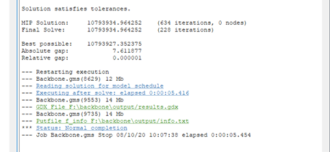
Open GAMS studio. Open the file “backbone.gms”, which is included in the backbone folder. In GAMS studio, you have a command line (marked with the big red arrow in the following picture) and a green start button (also marked in the following picture.

In the command line, you must type:
--input_file_excel="path/to/your_excel_file.xlsx" --tutorial=1
path/to/your_excel_file.xlsx must be replaced with the path, that leads to the excel input file you filled in the previous tasks. Make sure, the path is correct and leads to an existing backbone excel file, otherwise backbone will not work. It should also not contain spaces or special characters like ö/ü/ß etc.
For all tutorial runs, you have to use the flag --tutorial=1. For the case study runs, you must not use that flag.

Common errors
If backbone does not run sucessfully, there can be multiple reasons. On this page, we show you the most common ones. To see error messages, you have to look into the process log of GAMS Studio (on the right). Always start with solving the first error, that occured, because later errors might just be resulting from this first error.
- Incorrect path to backbone input excel: If the path to the excel file is incorrect or you forgot to save your excel file, you will get the error "Input excel not found Check that your input Excel is valid and that your file path and file name are correct". Check the path you gave in the command line.

- 'utf-8' codec can't decode/Error in embedded code section: Special characters in the input excel path can be a problem (ü/ö/ä/ß or space etc.). Copy your input file to a path without special characters.

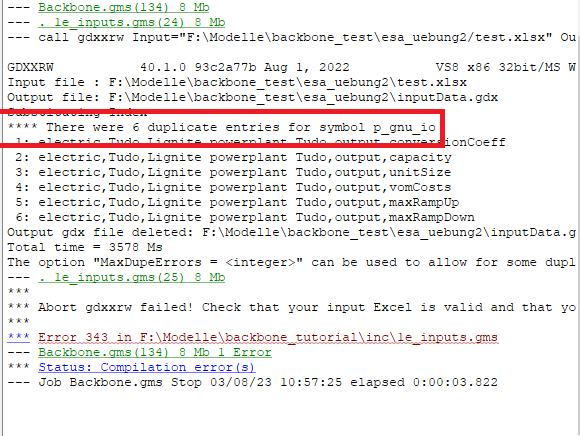
- Duplicates in the excel input file: Your input file must not contain duplicate entries. If it contains duplicate entries, you will get an error with the message like **** There were 6 duplicate entries for symbol p_gnu_io. Luckily, GAMS tells you, in which sheet the duplicates occur. Remove the duplicates to get backbone running.

- Domain Violation: This very common error shows that you refer to something in your sheets that was not defined before. Usually, this is provoked by spelling mistakes (e.g. power-plant instead of powerplant). Finding the causes of domain violation errors can be a little tricky. In GAMS studio you can click on the error message. Then, GAMS studio marks the table in the editor, in which the error occured. You then must compare the names of the units/grid/nodes in this table with the names defined in the inital parameter sheets (named only "grid", "node" or "unit", yellow) to find the spelling mistake.

- Unable to open input file: Backbone does not find all necessary files. This often happens, if something went wrong with the download of the backbone programme. You need the whole folder (not only the file backbone.gms). Repeat the download to fix this error.

Display and analyize results
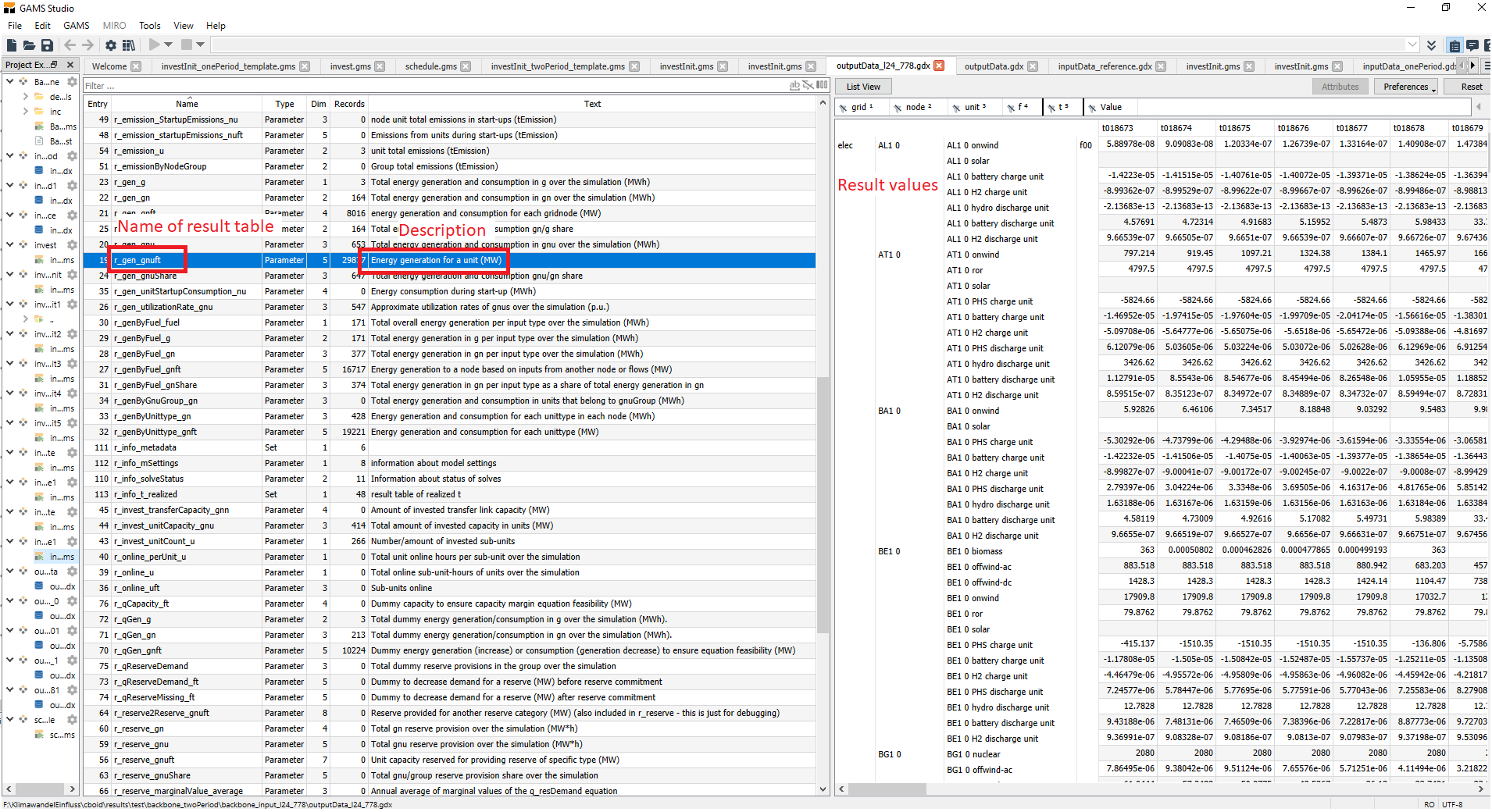
After sucessfully running backbone, you will find a file named "results.gdx" in the folder backbone/output. This is the main output file of backbone. It contains all results from the optimization. You can open it with GAMS studio to look into the results. On the left, you will see a table containing all result tables. Next to the tables, there is a description of the results table (maybe you have to enlarge this part of the window to see this information). If you click on a result table, it will be displayed on the right. There are a lot of very small numbers in the results. This is due to the solving algorithm. You can ignore every value, that is smaller than 1.

The gdx file provides a good overview over all results, however, it is not optimal to analysis results. Therefore, the most important tables are also saved as excel files. This tables are:
r_gen_gnuft - energy generation from a unit (MW)
r_invest_unitCount_u - number of invested units
r_state_gnft - node state at timestep t (MWh)
r_qgen_gnft - dummy energy generation/consumption at timestep t (MW)
r_cost_realizedCost - total realized system cost over the simulation (MEUR)
For the analysis of the first tutorial, we will only need r_gen_gnuft. The meaning of the other tables will be explained in further tutorials.
Note: On Mac and Linux machines, no Excel files are exported automatically. To manually export the sheets you need, use the Export button in GAMS studio.

Task: Plot your results
Solution: Plot your results

- Graphs should always contain axes labels and units
- Stacked area graphs are more insightful, if the units are sorted in a senseful way (e.g. base load plants at the bottom, peak power plants on top)