1. Preparation of input data
| Website: | RUB Moodle |
| Kurs: | Case Study "Novel flexibility options in the German electricity grid" (SoSe23) |
| Buch: | 1. Preparation of input data |
| Gedruckt von: | Gast |
| Datum: | Sonntag, 26. Juli 2026, 20:24 |
Case study description
Germany has stated to achieve climate neutrality by 2045. The electricity production thereby places a major role, as it holds a large share of the greenhouse gas emissions. Renewable technologies like solar and wind power can already produce electricity at low costs, but due to their weather dependency, they only provide electricity intermittently. This poses challenges to the grid operation, as it is more difficult to match the generation to the demand profiles. These challenges result in a need for flexibility options.
In this case study, the influence of two novel flexibility technologies on the German electricity system in 2045 are examined. The study is based on a model of the German electricity grid in 2013. After adapting the model to the target year 2045, the influence of wo different flexibility options shall be examined: hydrogen storage and elastic demand.
In this case study, you shall prepare input data three different scenarios:
- base case
- hydrogen storage scenario
- elastic demand scenario.
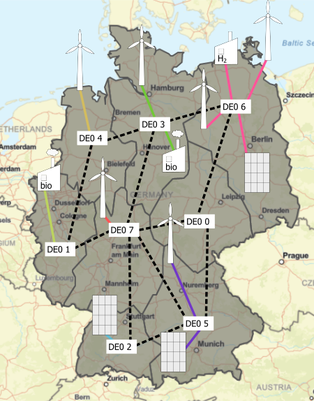
In the following figure, you can see the study area:
Base case preparation
For preparing the base case scenario, download the provided excel file “InputData_caseStudy.xlsx”. It contains a model of the German electricity grid for the year 2013. The model is in a time resolution of 6 hours, that means, every timestep t is representing 6 hours. The branch you started now, has two aims: first you shall familiarize yourself with the model. In a second step, you shall adapt the model to the target year 2045.Tasks: Understanding the model
Adapting the model for 2045
As you have seen in the previous question, a lot of things have to be adopted, when converting a model from 2013 to 2045.
We
will focus on two adaptions here: the available power plant park and
the demand. The technology costs in the model are already adopted to
2045. In the next to paragraphs you can find information on what has to be changed in your model.
Demand
Following projections by DENA [1], the demand in Germany
will rise by 43 %. Scale all the demand you find in the sheet ts_influx
in the model by this factor.
[1] Bründlinger, T. et. al. (2018): dena-Leitstudie Integrierte Energiewende. Edited by Deutsche Energie-Agentur GmbH (dena). Available online at https://www.dena.de/fileadmin/dena/Dokumente/Pdf/9261_dena-Leitstudie_Integrierte_Energiewende_lang.pdf, checked on 10/27/2022.
Power plant park
Look at the available power plants. Which of those will still be available in a climate neutral Germany in 2045? Think about both climate based and other political decisons, while excluding technologies like CCS. Disable all power plants which you expect to be not available anymore. Hint: It is not necessary to remove the powerplants from the excel file to fulfil this task. Make use of the parameters, backbone provides.
Run base case backbone
You should now have multiplied all demand (only the negative
numbers in ts_influx) by 1.43 and made all fossil power plants (lignite,
coal, oil, CCGT
and OCGT) and the nuclear power plants unavailable (set the parameter availabiltiy
in p_unit to 0). Now your model is adopted for the target year. Before
adding any new flexibility options, run the model once (change the path in the command line to your new input file). Remember to remove the "--tutorial=1" flag from the command line. After completion, copy all results from the backbone output folder and save them.
Hydrogen scenario preparation
In this scenario, you shall add hydrogen storages as a flexibility option. The following tasks and pages will help you prepare your input data.
Task: Implementation of hydrogen storage
The
storage of hydrogen in salt caverns is the most promising technology option.
Only the north of Germany has the geological potential to store hydrogen in
salt caverns. Therefore, you can find three hydrogen cavern storages in the
northern nodes DE0 3, DE0 4 and DE0 6. They are pre-implemented with a maximal storage
capacities of 7.73 PWh each [1]. To
produce hydrogen from electricity, we will use
electrolyses, to retransform the hydrogen to electricity, we will use
hydrogen
gas turbines. The implementation of hydrogen storages is very similar to
the implementation of battery storages.
[1] Caglayan, Dilara Gulcin; Weber, Nikolaus;
Heinrichs, Heidi U.; Linßen, Jochen; Robinius, Martin; Kukla, Peter A.;
Stolten, Detlef (2020): Technical potential of salt caverns for hydrogen storage
in Europe. In International Journal of Hydrogen Energy 45
(11), pp. 6793–6805. DOI: 10.1016/j.ijhydene.2019.12.161 
Data for hydrogen storage
Implement
an electrolyzer and a gas turbine in each of the three
northern nodes as invest unit with infinite investment potential and no
integer
investment (investMIP = 0). The discount rate is 7%, you find all other
necessary data in the table below. For
connecting the units to grids, refer to the sketch you prepared about
the batteries in DE0 3. If you cannot recall how to implement new investment units, refer to the tutorials.
Hint: As you may have noted, there is only one efficiency (eff00) in p_unit and no minimum operation point. This is due to the simplified representation of powerplants in this bigger model to save computational time (remember the different cases from exercise 1). You can just add the one efficiency given as eff00 and not provide a minimum operation point.
Second
Hint: You do not have to fill the column "UpperLimitCapacityRatio". For
further information, read the comment in the excel file.
|
|
Invest costs (€/MW) |
FOM costs (€/MWa) |
VOM costs (€/MWh) |
Lifetime (years) |
Efficiency (%) |
Unit size (MW) |
|
electrolyzer[1] |
2.7 * 105
|
9.4 * 103
|
1.2 |
30 |
78 |
1 |
|
Gas Turbine[2] |
8.5 * 105
|
2.1 * 104
|
2 |
30 |
62 |
1 |
[1] Child, Michael; Kemfert, Claudia; Bogdanov,
Dmitrii; Breyer, Christian (2019): Flexible electricity generation, grid
exchange and storage for the transition to a 100% renewable energy system in
Europe. In Renewable Energy 139, pp. 80–101.
DOI: 10.1016/j.renene.2019.02.077, Gorre, Jachin; Ortloff, Felix; van Leeuwen,
Charlotte (2019): Production costs for synthetic methane in 2030 and 2050 of an
optimized Power-to-Gas plant with intermediate hydrogen storage. In Applied
Energy 253, p. 113594. DOI: 10.1016/j.apenergy.2019.11359
[2] Moles, C.; Sigfusson, B.; Spisto, A.; Vallei, M.; Weidner, E.; Giuntoli, Jacopo et al. (2014): Energy Technology Reference Indicator (ETRI) projections for 2010-2050. Luxembourg: Publications Office (EUR, Scientific and technical research series, 26950)
Run hydrogen scenario backbone
Now run the model. If you ran another scenario
before, check, whether you have disabled the other flexibility options
(elastic demand) before running this model. Remember to remove the "--tutorial=1" flag from the command line. After completion, copy all results from the backbone output folder and save them.
Elastic demand scenario
The second flexibility option will be to consider elastic demand. Elastic
demand
reflects the fact, that people might be willing to change their
consuming
behaviour such that in hours with very high demand, they consume less
instead
of paying really high energy prices. We can use this behaviour to lower the costs of our system. The following pages will show you how to include elastic demand into your system.
Task: Calculation of Value of Lost Load
Implement elastic demand and run backbone
To implement elastic demand in backbone, we will use the "penalty" paramter of backbone. This parameter allows backbone to not meet demand and instead pay a preset penalty. The standard penalty value for not meeting demand is 109 €/MWh. We can change this value by adding the option --penalty=value (in €/MWh) to the command line.
You shall now run your model three times: once
with the average VoLL of 18.92 €/kWh, once with the maximum VoLL
of 58.29 €/kWh and once with the minimum VoLL of 6.40 €/kWh (pay attention to the units). Remember to
disable the hydrogen units and to remove the "--tutorial=1" flag from the command line. For each run, copy all results from the backbone output folder and save them.
Preparation for analysis of results test
To be sure that you have correct results to go into the final test, we will provide you with some values to check your solution. In the result.gdx you achieved for each scenario, there is a variable "r_cost_objectiveFunction_t". In the following table you find the values this variable should have (little deviations are ok). If you recieved another value, check whether you followed all instructions for the preparation of the input data correctly.
| scenario | base | hydrogen case | elastic demand - average VoLL | elastic demand - min VoLL | elastic demand - max VoLL |
| r_cost_objectiveFunction_t | 196005 | 85935 | 192138 | 172628 | 196005 |
In the final test, you will be asked to upload four plots. To save time, you should prepare them before hand. The plots are:
- For the base case, plot the storage state of the node DE0 5 battery over the year (as reported in r_state_gnft).
- For the base case, plot the production of the renewable generators over the year (as reported in r_gen_gnuft).
- A diagramm comparing the total realized costs between the 3 cases you modeled (base case, hydrogen storage and elastic demand with average VoLL). You can neglect the results for minimum and maximum VoLL here.
- A diagramm comparing the number of invested units (grouped by carrier: solar, wind, battery, hydrogen storage) of the 3 cases you modeled (as definded above). Backbone does not directly provide this information, therefore you will have to work a little with the information provided in r_invest.
Be careful to add axes labels and units.
Onshore wind is shortened with onwind, offshore wind with offwind. There are two types of offshore wind (ac and dc), this referes to the type of connection they have with the mainland (alternate current or direct current). For the analysis, this does not matter, you can just add all types of wind to the carrier wind.